CS - SDK

csSDK (ConverSight Software Development Kit) is an optimized and updated version of ConverSight Library. Functionalities are same as ConverSight Library. But it is a combination of low code and no code environment. It is enhanced in such a way to optimize the time taken for every action.

Using the csSDK, a range of actions can be executed including connecting datasets, viewing dataset details and metadata, retrieving group and role information, running queries and accessing pinned Storyboards. In the future, the csSDK will enable the creation, updating and deletion of Proactive Insights, Relationships, Drilldowns, smart analytics, smart column and smart query through Notebook.

---

The csSDK Library has two powerful functionalities that serve as its backbone:

• Dataset Functionalities

• Pinboard Functionalities

Dataset Functionalities

Let’s take a closer look at Dataset Functionalities, which enable users to work with datasets. To start with csSDK Library in Jupyter Notebook, first import dataset from csSDK Library.

from csSDK import Dataset
# This will import all the dataset from the csSDK Library

When you use ConverSight Library without entering a dataset ID, it connects to all the datasets in the library. However, about the CS-SDK, this will necessitate a specific dataset ID.

ds = Dataset("6412ae74-N3VuSsa4m")
#where "6412ae74-N3VuSsa4m" is the dataset ID

Dataset Load

NOTE
The keyboard shortcut Shift + Enter is utilized to execute a cell.

Available Methods in Dataset

Pressing the Tab button on an object or function displays a list of the available functions. List of available methods for dataset are shown in the below screenshot.

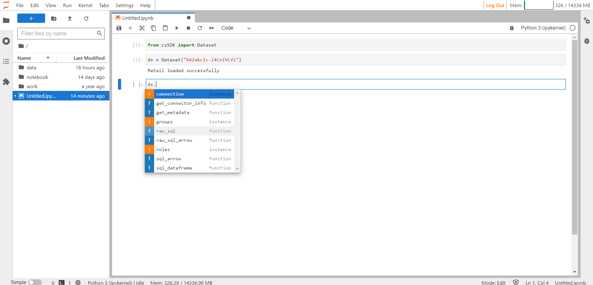
Available Functions in CS SDK

NOTE
The keyboard shortcut Shift + Tab is used to view the help guide for a method.

Connection

The purpose of a connection is to establish a link to datasets, enabling users to access information about tables and execute queries. There are several methods that can be found in a connection, such as:

• execute

• get_tables

• get_table_details

• load_table

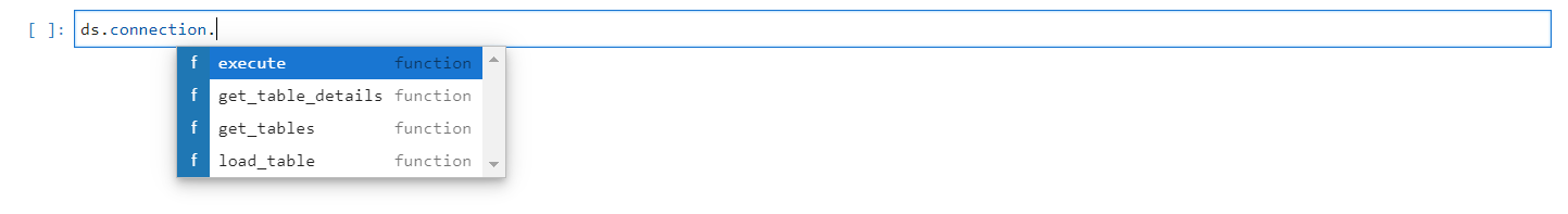
Available Functions in Connection

Execute: The execute() method is utilized to run a query on tables and provide the results to users. It can take either SQL query or object as arguments but any one is mandatory

Sql_ds=ds.connection.execute("""SELECT
      round(
        sum(coalesce(m_642abc55_RetailSales."m_revenue", 0)),
        4
      ) AS "label_RetailSales.revenue",
      m_642abc55_RetailSales."m_buyer" AS "label_RetailSales.buyer",
      round(
        sum(coalesce(m_642abc55_RetailSales."m_units", 0)),
        4
      ) AS "label_RetailSales.units"
    FROM
      m_642abc55_RetailSales
    GROUP BY
      m_642abc55_RetailSales."m_buyer",
      m_642abc55_RetailSales."m_buyer"
    ORDER BY
      m_642abc55_RetailSales."m_buyer",
      m_642abc55_RetailSales."m_buyer"
    LIMIT
      50002""")

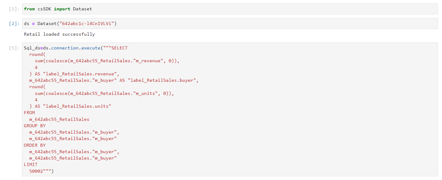
Executing a SQL Query

Get Tables: The get_tables() method enables users to obtain a list of all the tables that exist within a database, including their corresponding table ID. This information can be useful for users to gain insight into the available tables.

tables=ds.connection.get_tables()

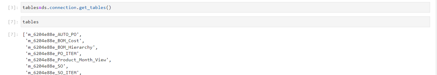
List of Available Table in the Dataset

Get Table Details: The user can use get_table_details() method obtain information regarding the column and data types of the given table. It is essential to have the table name to access the details, as an error would be generated otherwise.

The user can refer to the help guide to determine the necessary arguments required for utilizing the method.

Get Table Details Help Guide

Get Table Details Method

Load Table: The load_table() method allows the user to load a table into a database. If the table already exists and its size matches, the data in the table will be appended. However, if the size does not match, an error will be thrown. On the other hand, if the table name does not exist, a new table will be created with that name and the data will be loaded into it.

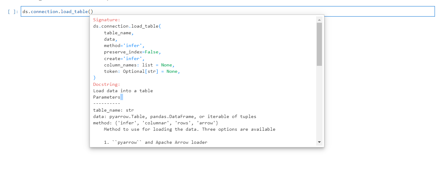
Load Tables Arguments

ds.connection.load_table(table_name="Retail", data=df)

Load Table

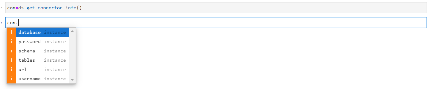
Get Connector Information

The get_connector_info() method involves in extracting information of the connector and presenting it to the user in a comprehensible format, which includes information such as the name of the database, the schema, the tables, the URL and the username. It is noteworthy that in many cases, the password is obscured as a security measure, appearing as a series of asterisks (*****).

con=ds.get_connector_info()

The available methods in get_connector_info() are:

• database

• password

• schema

• tables

• url

• username

Get Connector Information Methods

Database: The database retrieves the name of the database that is currently connected.

Database Method

Password: For security purposes, the password retrieves a series of asterisks representing the password that has been given to the database.

Password Method

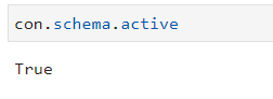
Schema: The schema provides information about the connector’s schema. The avaialble methods under schema are:

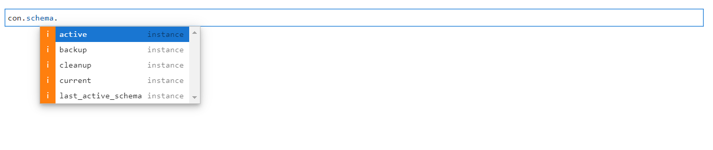
Schema Methods

Method	Description
active	The active method indicates whether a schema is currently active or inactive.
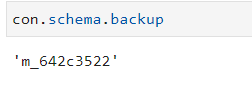
backup	The backup method shows the ID of the backup schema.
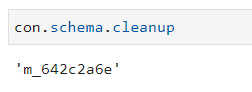
cleanup	The cleanup method shows the ID of the deleted schema.
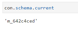
current	The current method shows the ID of the currently running schema.
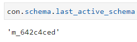
last_active_schema	The last active schema shows the ID of the last active schema.

Tables: The table method shows the list of tables that are available in the dataset.

Table Method

URL: The url method shows the URL utilized for establishing a connection to the dataset

URL Method

Username: The username displays the user associated with the dataset.

Username Method

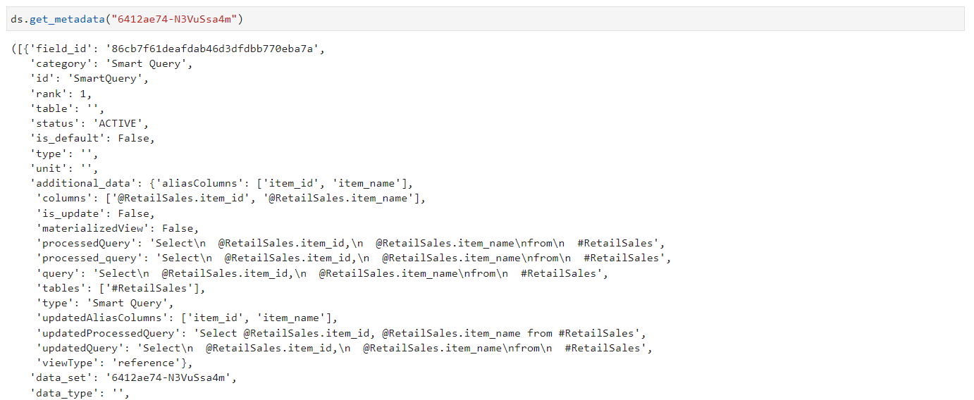
Get Metadata

The get_metadata() method retrieves comprehensive information about a dataset, including all properties of every table and column. This method can be useful for data analysts and developers who need to understand the structure and content of a dataset in detail. Dataset ID is mandatory for this method.

ds.get_metadata("6412ae74-N3VuSsa4m")
# where "6412ae74-N3VuSsa4m" is the Dataset ID

Metadata Method

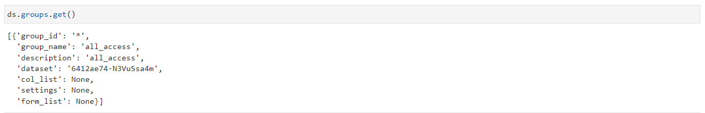
Groups

The group method contains only the get method, which displays the group ID, group name, description, dataset, column list, settings and form list. The user can use this method to understand about the permission and access given to the database.

ds.groups.get()

Groups

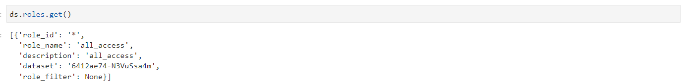
Roles

The roles method retrieves information about the roles associated with a dataset, including the role ID, name, description, dataset and role filter. This method is useful for understanding the permissions and access of the roles. By using the roles method and the get function, developers and data analysts can quickly retrieve important information about the roles defined within a dataset.

ds.roles.get()

Roles

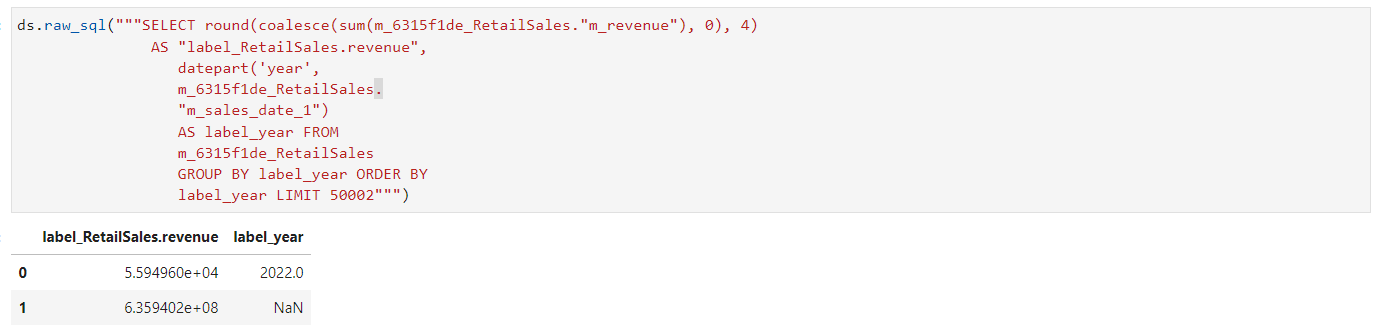
Raw SQL

Raw SQL is a fundamental and low-level approach to interacting with databases. The raw_sql() method is used to process the SQL queries and display the results in a tabular format. This method is useful for advanced users who need more granular control over their database interactions and who are comfortable working directly with SQL queries. The raw_sql() method may become a more integral component of larger database interaction workflows.

ds.raw_sql("""SELECT round(coalesce(sum(m_6315f1de_RetailSales."m_revenue"), 0), 4)
                    AS "label_RetailSales.revenue", 
                        datepart('year', 
                        m_6315f1de_RetailSales.
                        "m_sales_date_1")
                        AS label_year FROM 
                        m_6315f1de_RetailSales
                        GROUP BY label_year ORDER BY
                        label_year LIMIT 50002""")     

Raw SQL Method

Raw SQL Arrow

Arrow SQL can be used alongside normal SQL to improve the performance and efficiency of data processing tasks. Arrow SQL can be used to transfer data between different systems without the need for expensive data conversions, which can save time and resources. Additionally, Arrow SQL can be used to optimize queries by leveraging the highly efficient columnar format, resulting in faster query times and improved performance. The method raw_sql_arrow() accepts raw SQL as input and processes it, producing output in a standard columnar format.

ds.sql_arrow("""SELECT round(coalesce(sum(m_6315f1de_RetailSales."m_revenue"), 0), 4)
               AS "label_RetailSales.revenue", 
                  datepart('year', 
                  m_6315f1de_RetailSales.
                  "m_sales_date_1")
                  AS label_year FROM 
                  m_6315f1de_RetailSales
                  GROUP BY label_year ORDER BY
                  label_year LIMIT 50002""")

Raw SQL Arrow Method

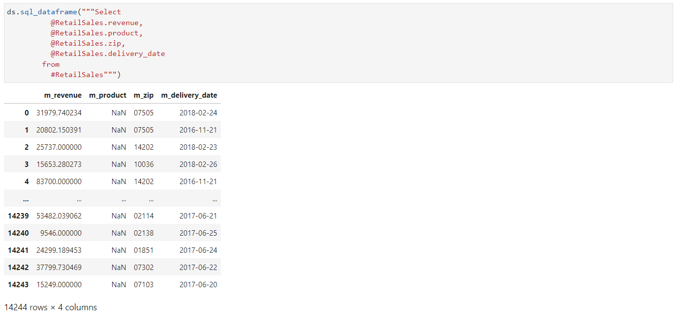
SQL Dataframe

The method sql_dataframe() takes a SQL query as input, where @ is used to refer to a column and # is used to refer to a table. It processes the query and returns the resulting data in a tabular format.

ds.sql_dataframe("""Select
          @RetailSales.revenue,
          @RetailSales.product,
          @RetailSales.zip,
          @RetailSales.delivery_date
        from
          #RetailSales""")

SQL Dataframe Method

SQL Arrow

The sql_arrow() method accepts a SQL query as input, with @ used to represent columns and # used to represent tables. It processes the query and returns the data in a standard columnar format, which is known for its efficiency and faster processing time compared to traditional SQL methods.

ds.sql_arrow("""Select
          @RetailSales.revenue,
          @RetailSales.product,
          @RetailSales.zip,
          @RetailSales.delivery_date
        from
          #RetailSales""")

SQL Arrow Method

Pinboard Functionalities

Let’s take a closer look at Pinboard Functionalities, which enable users to work with datasets. To start with csSDK Library in Jupyter Notebook, first import solution from csSDK Library.

from csSDK import Solution
# This will import Solution from the csSDK Library

Once an object is instantiated with the Solution() method, pressing the tab key reveals the list_templates() method, which can be used to retrieve a comprehensive list of available templates on the platform and their respective versions.

sn = Solution()
sn.list_templates()

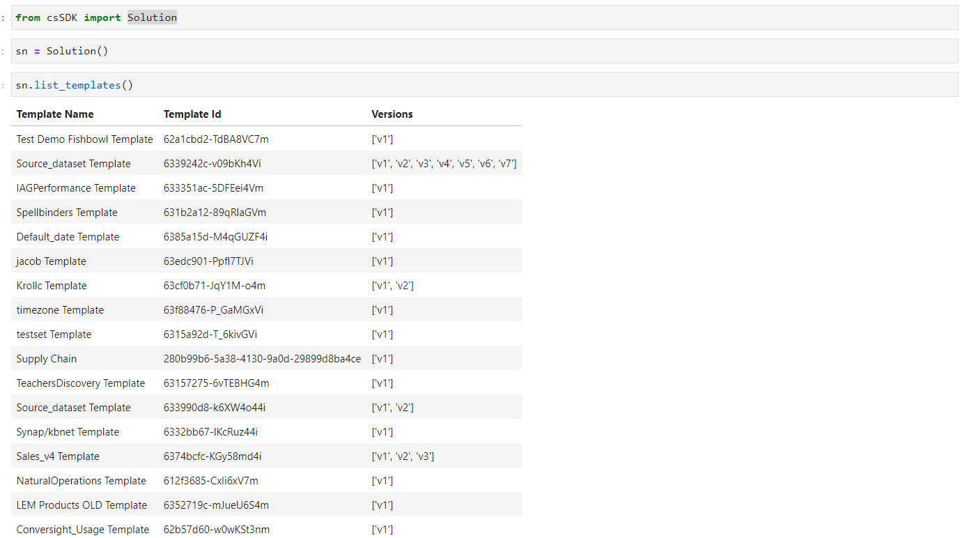
List of Available Templates

To access Pinboard Functionalities, users can pass the template ID as a parameter to an object, which can then be utilized for Pinboard features.

sm=sn["280b99b6-5a38-4130-9a0d-29899d8ba4ce"]

Available Methods in Pinboard

Pressing the Tab button on an object or function displays a list of the available methods. List of available methods for pinboard are shown in the below screenshot.

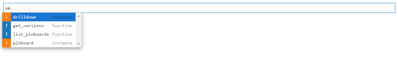
Pinboard Methods

Get Versions

The get_versions() method shows all available versions of a specified template, along with their corresponding templates.

sm.get_versions()

Get Version Method

List of Pinboards

When a version is passed as an argument, the list_pinboards() method displays the available pinboards.

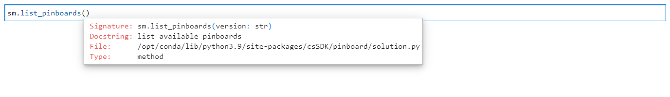
Arguments for List of Pinboard

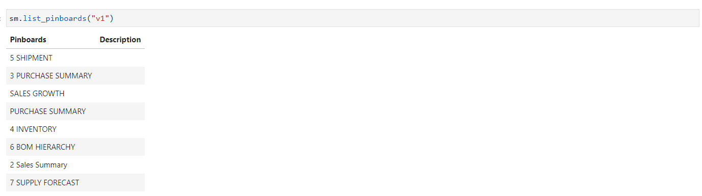
List of Pinboards

Pinboards

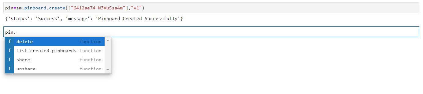
The Pinboard method only contains the create() function, which requires arguments for dataset ID and version. The create() function in the Pinboard method creates a pinboard within the specified dataset.

sm.pinboard.create()

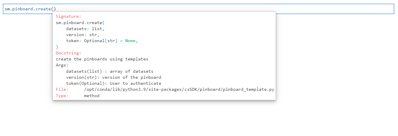
Arguments for Create Pinboard

Pinboard Created

After the pinboard is created, the assigned object displays a list of methods, which are listed below:

• list_created_pinboards

• share

• unshare

• delete

Pinboard Methods

List of Created Pinboards: To display the ID and name of a pinboard that has been created, the method list_created_pinboards() can be utilized.

pin.list_created_pinboards()

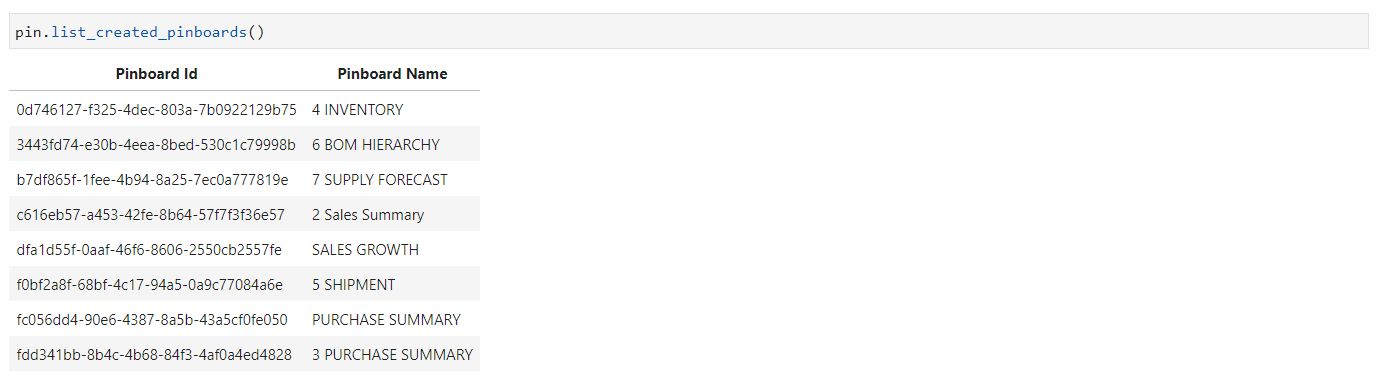
List of Created Pinboards

Share: The method share() allows for the sharing of a pinboard with one or more users by including their email addresses. However, it is important to note that the recipient(s) must also have access to the dataset in order for the pinboard to be successfully shared.
The required arguments for the method “share()” are:

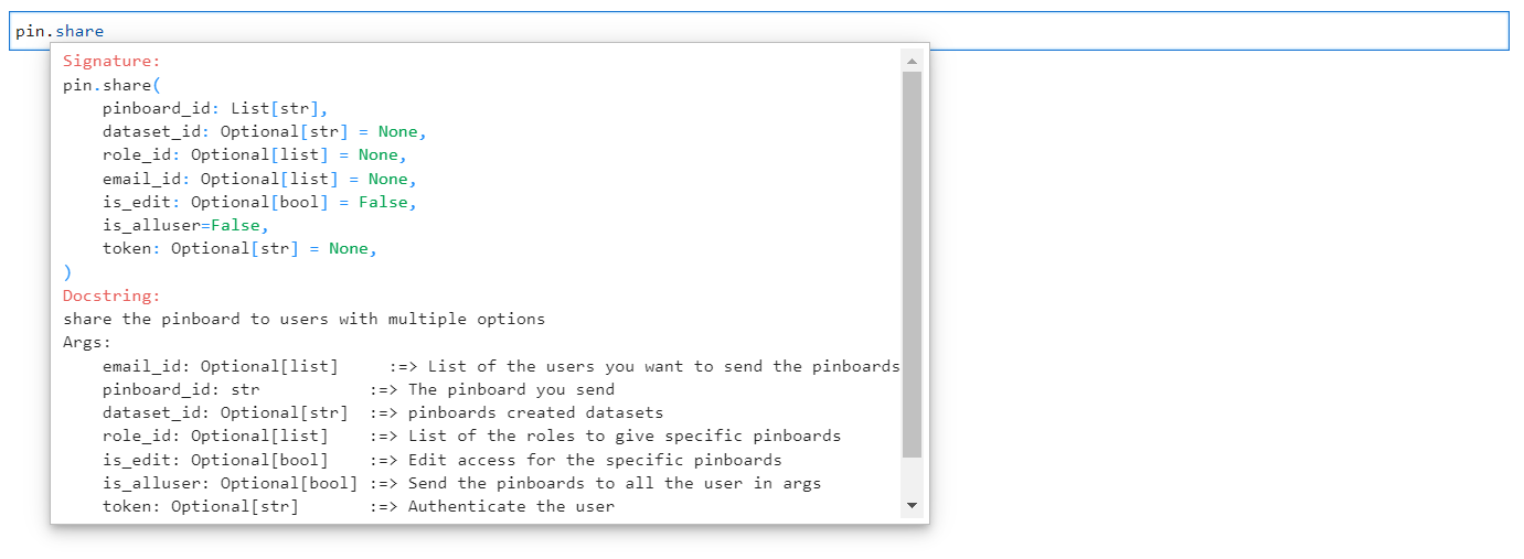
Arguments for Share method

pin.share(email_id=["admin123@conversight.ai"],pinboard_id=["c616eb57-a453-42fe-8b64-57f7f3f36e57"])

Pinboard Shared

Unshare: To remove a shared pinboard, the unshare() method requires the ID of the pinboard as well as the email address of the user with whom it was shared. The required arguments for the method “share()” are:

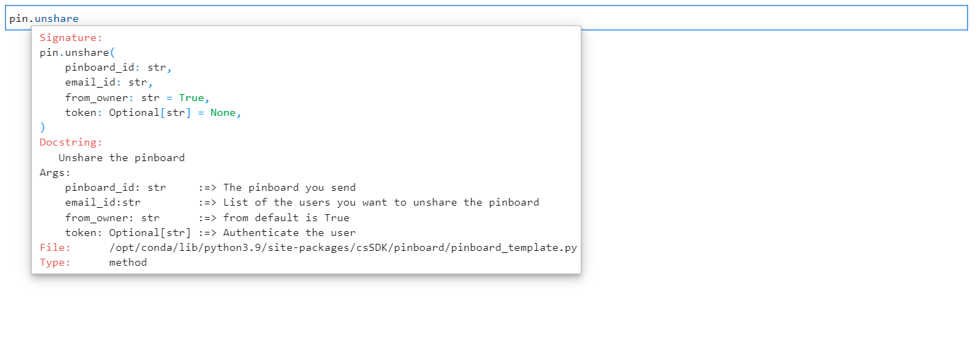
Arguments for Unshare method

pin.unshare(email_id="admin123@conversight.ai",pinboard_id="c616eb57-a453-42fe-8b64-57f7f3f36e57")

Pinboard Unshared

Delete: The delete() method is responsible for deleting a pinboard, along with any copies of the same pinboard that have been shared with other users. It takes pinboard ID as arguments.

Pinboard Deleted

Using the csSDK, a range of actions can be executed including connecting datasets, viewing dataset details and metadata, retrieving group and role information, running queries and accessing pinned Storyboards. In the future, the csSDK will enable the creation, updating and deletion of Proactive Insights, Relationships, Drilldowns, smart analytics, smart column and smart query through Notebook.

V2 Data Management with csSDK

In ConverSight, datasets exist in two versions: V1 and V2. The primary difference between these versions lies in how data and metadata is handled:

• V1 Dataset: Uses MapD as storage, requiring predefined metadata before writing data. Without metadata, the system cannot recognize or process the table.

• V2 Dataset: Is serverless and uses object stores such as S3, Blob or GCS for storage. This allows users to write data directly to storage, with metadata generated later to ensure accessibility in Athena.

Managing V2 datasets involves two processes: Data Storage and SME creation (metadata management). The raw data is stored in object storage like S3, Blob or GCS, allowing users to write data directly without requiring predefined metadata. Separately, metadata is created using the csSDK.Semantics module, ensuring that the data is structured, recognized and ready for querying. This separation provides flexibility, enabling data to be stored independently while metadata is managed and updated as needed.

Writing Data to Object Storage

The process involves preparing and writing the dataset into object storage. It includes importing necessary libraries, reading and converting data, determining the storage path and storing the dataset in the appropriate location. The following are the steps:

Step 1: To begin, we need to import the necessary libraries that allow us to manage metadata and interact with cloud storage.

For Example,

from csSDK import Semantics, ObjectSchema, Category, SemanticObject, Mode 
from google.oauth2 import service_account 
from google.cloud import storage 
import base64 
import json 
import polars as pl 
import pyarrow as pa 

In the example above, the essential imports include the csSDK module, which offers classes for defining and managing metadata (such as Semantics, ObjectSchema and SemanticObject). Additionally, Polars and PyArrow are imported to handle data processing, enabling efficient dataset transformations.

The data storage details depend on the user’s preferred storage system. In the example above, we used the Google Cloud SDK (google.oauth2 and google.cloud.storage) to enable authentication and interaction with object storage.

Importing Libraries

Step 2: Specify the table name from the imported data storage, which will be used throughout the process of metadata creation and management. The table name must be in lowercase and can only contain letters, numbers and underscores (_). It should remain consistent when writing data and defining metadata to avoid mismatches.

For Example,

table_name = 'sales_order_details'

Step 3: Read the Parquet file containing the data and convert it into the Apache Arrow format. Parquet is a commonly used format for storing structured data efficiently. Load it using Polars (pl.read_parquet()) and then convert it into Apache Arrow format, which is required for metadata definition.

For Example,

df = pl.read_parquet('sales_order_details.parquet') 
arrow_data = df.to_arrow()

Step 4: The storage path is determined dynamically using the Semantics module.

For Example,

sm = Semantics(dataset_id) 
sm.upload_path 

Upload Path

ConverSight provides a bucket path for users to store their datasets efficiently in object storage. This ensures that all data is properly structured and accessible for further processing. Users also have the flexibility to configure and use their own object store, which will be mapped to the dataset during setup.

This step retrieves the object storage path, following the format:

gs://{bucket_name}/data/{org_id}/{dataset_id}/delta/{table_name}

This ensures that the table is stored in the correct location within the object storage.

Step 5: Once the storage path is identified, write the data into object storage which in this case is the Google Cloud Storage. This operation saves the dataset in Delta format using the object storage path. The storage_options parameter ensures proper authentication with a service account (your.json). If users are using their own data store, they should use their respective configuration settings. The mode=”overwrite” setting ensures that any existing data is replaced with the new version.

df.write_delta( 
    f"gs://{sm.upload_path}{table_name}", 
    storage_options={"serviceAccountKey": "your_config.json"}, 
    mode="overwrite" 
) 

In the example above, we used Polars to write data to GCS with a service account.

NOTE
The table and column names must be in lowercase when written into storage.

Creating and Publishing Metadata

Once the data is stored, metadata must be created and published to make it accessible in ConverSight. This process includes defining metadata, creating SME objects, configuring metadata actions and publishing SME. The following are the steps:

Step 6: After writing the data, extract schema from the Apache Arrow table format. The schema defines the structure of the table, including column names and data types. This is necessary for creating metadata that accurately represents the stored data.

For Example,

schema = arrow.schema 

Step 7: Define the metadata object, which serves as a representation of the table structure.

This ObjectSchema includes three key attributes:

• name – The name of the table (sales_order_details).

• object_schema – The extracted Apache Arrow schema of the table.

• category – The type of object (TABLE or ANALYTICS).

The category type determines how the table is used within ConverSight. For raw physical tables, Category.TABLE is used and Category.ANALYTICS is used for analytical processing, allowing optimized storage and faster performance for complex queries.

For Example,

object_schema = ObjectSchema(name=table_name, object_schema=schema, category=Category.TABLE) 

Step 8: Once the structure is defined, the object is initialized to prepare it for metadata configuration.

For Example,

obj = ObjectSchema(name=table_name, object_schema=schema, category=Category.TABLE)

Step 9: To create metadata, define a SemanticObject that contains the table schema and specify the Mode.create option. This prepares the table in a “created” status, meaning it’s ready to be published but not yet active in the system. You can also specify Mode.delete to remove metadata if needed. Both actions can be set up in a single configuration list.

For Example,

configure = [SemanticObject(object=obj, mode=Mode.create), 
            SemanticObject(object=obj, mode=Mode.delete)] 
sm.configure(objects=configure) 

Metadata Creation

To delete metadata, use the same structure but change the mode to Mode.delete. This removes the metadata, making the table inaccessible for queries.

For Example,

configure = [SemanticObject(object=obj, mode=Mode.delete)] 
sm.configure(objects=configure) 

NOTE
Multiple tables can be created or deleted at the same time by specifying multiple SemanticObject configurations in a single configure list. Since an update option is not available, any changes to the metadata require deleting the existing table and creating it again with the updated configuration.

Step 10: Once data is created or deleted, changes must be published to synchronize with the stored data. This is done using the publish_sme() function.

For Example,

sm.publish_sme() 

SME Publish

This operation synchronizes the metadata with the stored data and ensures that:

• All tables and objects are properly registered in the dataset.

• The schema matches the stored data, avoiding discrepancies.

• The metadata is available for querying in Athena and ConverSight.

The publish process verifies if each table exists in storage and updates the Delta table version written in the object store:

• If a table exists, its metadata is updated.

• If a table is missing, its metadata is deleted.

• If a table is missing in storage, an error is raised.

This ensures that the dataset remains consistent and up to date.

By following these steps, users can store data in object storage, define metadata dynamically and publish it for use in ConverSight. This approach provides greater flexibility and scalability, making metadata management more efficient and adaptable to changing data requirements.